Molecules in Motion: The Convection Express, The Diffusion Local
Every CVD reactor puts gases in somewhere, takes them out, and hopes that somehow the relevant molecules get to the place where a film is supposed to form, so that they can be incorporated into it [and byproducts can be carried away]. Thus understanding of the reactor requires that we know how molecules move from one place to another in a gas.
In our everyday lives we are aware of the motion of gases: the wind blows carrying leaves away from neatly raked piles as it transports heat from the tropics to the poles. We usually think of this motion in terms of an overall velocity carrying all the molecules in a region together: convection. This sort of motion of gases can be described in terms of a velocity field -- a vector associated with each point in space occupied by the gas, describing the local average speed and direction of the molecules in the gas. An infinitesimal particle caught in the gas would follow a streamline through space; the collection of streamlines defines the paths of packets of gas in the flow. We can imagine that the flow might be very complex. For example, let's examine a fairly complex geometry which might arise in a CVD context: a gas flowing through a channel defined by impermeable walls:
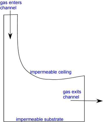
The streamlines (the idealized lines describing the direction of fluid flow at each location) can’t pass through the walls, so they might look something like:
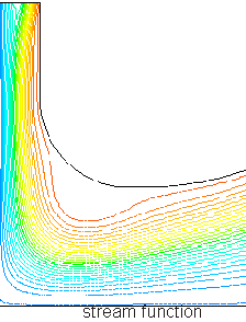
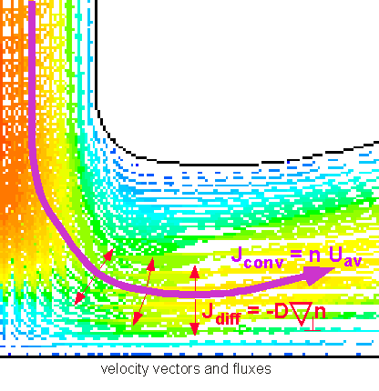
Each contour of stream function shows the path of a test particle through the gas from the top left to the bottom right. Velocity increases where the gas passes through narrow regions (the red at the top) and decreases in open areas (light and dark blue), so that the total molecules passing into and out of any region are equal (in steady-state flow):
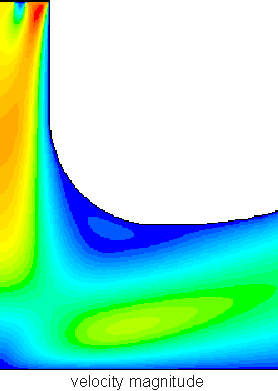
The velocity field above is pretty complex (knowledgable readers will recognize boundary layer formation, incipient separation and recirculation), and much more complex flows are not only possible but common. We'll discuss some simple methods of figuring out what the velocity fields are later; for the present, assume that we know where the fluid goes and how fast. Our goals is to figure out how stuff moves in the chamber: to find the various convective fluxes: the amount of mass, momentum, or energy carried by the fluid as it moves. If we knew what the velocity field was, would we know the flux as well? To figure this out we need to work out an expression for the convective flux.
Convective Flux
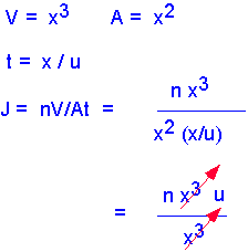
In formal mathematical terms, the flux is the amount of stuff (mass, momentum, etc.) carried across a plane by a flow per unit time. Consider an infinitesimal packet of stuff. The amount of stuff in the packet is the concentration "n" multiplied by the volume of the packet V.
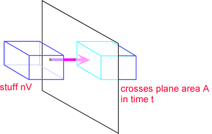
If we assume the characteristic length of a packet of stuff is x, then the volume scales as the cube of x, and the area as the square. The time required to move the packet through the plane scales as the size of the packet x, divided by the velocity of the packet u. Thus the flux is the (stuff per unit area per unit time). If we substitute our expressions for stuff, area, and time, we find that reassuringly the scale factor cancels: the flux is the product of concentration and velocity, independent of packet size so long as it is small enough that velocity doesn't vary across the packet.
So we see that to figure out how much stuff is being moved around, we need to know both the velocity field and the concentration field -- the concentration of whatever we're interested in as a function of position. However, in CVD we are generally dealing with an impermeable substrate (e.g. a silicon wafer), through which the fluid cannot pass. This can be seen in the images shown above: the stream lines never "touch" the walls. Thus convective flux to the substrate is always 0: convection alone cannot lead to deposition of a film on a solid substrate. We need to have some sort of transport mechanism that carries material "across" streamlines:
This mechanism is provided by molecular diffusion. Diffusion turns out to be very important in many ways in understanding CVD processes. Not only does it provide a mechanism for getting stuff to the surface; it is often the dominant transport mechanism in practical reactors and processes. Thus we'll spend quite a bit of time and effort to understand the role diffusion can play in transport. First we need an expression for diffusion flux, corresponding to that obtained above for convective flux.

Diffusive Flux
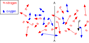
Diffusion is the macroscopic result of random thermal motion on a micoscopic scale. For example, in the diagram at right, oxygen and nitrogen molecules move in random directions, with kinetic energy on the order of kT. If there are more oxygen molecules on the left side of the plane A-A than on the right, more molecules will cross to the right than to the left: there will be a net flux even though the motion of each individual molecule is completely random.
The flux is proportional to the gradient in concentration (molecular or molar):
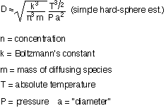
This is often known as Ficke’s Law. A simple estimate of the diffusion constant D is obtained by assuming that the molecules striking the plane A-A last collided one mean free path to each side, and move with mean thermal velocity (see kinetic theory for these terms). For "self-diffusion" (e.g. O[18] in O[16]) the form below is a reasonable approximation:
Typical values of D:
0.1 to 1 cm2/s @ 1 atmosphere (760 Torr)
75 to 750 cm2/s @ 1 Torr
NOTE: D is proportional to (1/P) where P is the pressure. For CVD the diffusivity can vary tremendously at low pressures.
The expressions above are fine for components present in small concentrations (infinitely dilute case). When the concentration is not negligible we must recall the constraint that the pressure (and thus total species concentrations) are constant everywhere. As a consequence, in for example a two-component mixture, if species 1 diffuses to the left, species 2 must diffuse to the right. D becomes the "binary diffusivity". A very rough estimate of binary diffusivity is obtained by using the RMS molecular diameter and the effective mass:

The Diffusion Equation
It would be nice to have a general way of describing how diffusion moves things around. The diffusion equation helps us find the concentration profiles and fluxes corresponding to a given set of boundary conditions.
Consider a volume from (x) to (x+dx) with transport only by diffusion. The change in the number of molecules with time is the difference between the flux going in and the flux going out, assuming molecules are not generated or lost in the volume.
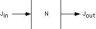
By using the Ficke's law expression for the flux, we can relate the change in concentration to the derivatives at the edges of the region.
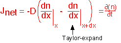
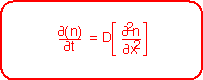
By expanding the derivative at x+dx to first order in the derivative at x, we can derive the Diffusion Equation, which describes the relationship between the spatial and temporal behavior of concentration:
Some Solutions to the Diffusion Equation
The general solution to the one-dimensional diffusion equation is the rather nasty infinite summation:
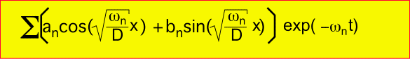
Here the “w’s” are "frequencies" (note their dimension is 1/time) determined by the boundary conditions, and the sum runs from n=0 [constant term] to infinite. Note that since the frequencies are of dimension (1/t) we can also consider them to be characteristic times, so that each term is of the form of a function of x/(Dt)1/2. We'll have more to say about that particular form in a moment.
Many practical situations can be approximated by two extreme cases:
1: fixed total amount of stuff, semi-infinite region:
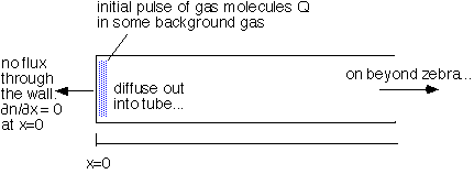
with solutions of the form:
2: fixed concentration at one boundary, semi-infinite region:
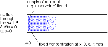
with solutions of the form:
Here erfc is the complementary error function, (1-the integral of a Gaussian).
Return to Tutorial Table of Contents
Book version of the CVD Tutorial