Some Useful Tools:
The source integrals and force relations
Daniel M. Dobkin
May 2007
A and Φ
Electromagnetism is the effect of charged particles (typically electrons and protons in the ordinary world) on other charged particles. These effects can be regarded as resulting from the action of a vector and scalar potential created by one charge and propagating to the location of the other charge. The potentials result from the charges and their motion. Moving charges create current, which is a vector with a direction at each point in space. We will usually characterize the charge and current as densities (coulombs/cubic meter and amps/square meter, respectively).
A brief notational digression: we will use boldface symbols for vectors (objects that have a direction) and italic for scalars (variables that have a numerical value but not a direction in space).
Every current creates a vector potential A that points in the same direction the current points in. The potential propagates away in all directions at the speed of light, with its amplitude falling inversely with distance. Charges work the same way -- except that charge is a scalar, rather than a vector like current, so the result is the scalar potential. (As we noted before, one can combine the current and charge into a relativistic four-vector that acts as the source of the relativistic potential composed of the spatial components (A) and the timelike component Φ, but in this discussion we'll take a non-relativistic viewpoint.) We can summarize these remarks in the source integrals:
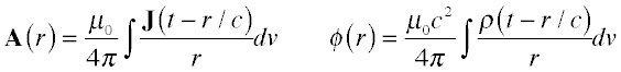
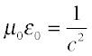
In these expressions, the integrals over current density J and charge density ρ are to be regarded as taking place over all the region we're interested in; for example, if we're figuring out how much power is radiated by an antenna we'd integrate over the whole antenna structure. The quantity r is the distance between the place where the charge or current is and the place where we're trying to find the potentials. We've introduced two constants: c is as usual the speed of light, 300,000 km/s, and μ0 is the magnetic permeability of vacuum, defined to be 4π x10-7 Henry/meter. While we find the use of the permeability convenient, it is entirely equivalent to use the dielectric permittivity ε0; they are related by:
Notice that the current or charge is taken at an earlier time t-r/c: that is, we assume the potential takes a while to get to where we are looking, traveling at the speed of light. This is known as a retarded potential. It looks innocent enough, but making this statement is actually equivalent to making a statement about the remainder of the universe, as Feynman and Wheeler showed in the late 40's. One can also formulate electrodynamics using both retarded and advanced potentials -- this is of great philosophical interest, and Mead spends some time investigating the consequences of such an approach, but it isn't terribly relevant for getting answers out of the sort of ordinary problems of interest when we're doing engineering. We'll just let time go forward. (If you want to know more about time asymmetry and irreversibility, check out both Mead's book and the very interesting Order Out of Chaos by Prigogine and Stengers.)
So if you know how the currents and charges are distributed you can find the potentials due to these charges at any location. We can equivalently require that the potentials satisfy the wave equation:
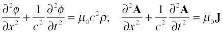
with appropriate boundary conditions. (We've shown the one-dimensional version; in two or three dimensions, we must employ the Laplacian operator rather than a simple derivative.) This is an entirely equivalent procedure and can be more convenient when the boundary conditions are easy to establish and the charge distribution hard.
For electrical engineering purposes, the result of these potentials is the total electric field:
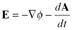
In many cases in electrical engineering, we are dealing with induced voltage on a metal object (e.g. an antenna or inductor, etc.). For reasonably high frequencies, we can assume that all the currents and charges are confined to the surface of the metal object, and we adjust those currents and charges until the net electric field is approximately zero inside of the metal. The difference in voltage between two points on the metal object -- the voltage we would measure if we applied two probes that draw no current and are not exposed to whatever external fields are present -- is the difference in the scalar potential between the two points.
The force on an individual particle of charge q is the product of charge and field, qE. One can equivalently regard the vector potential as a collective contribution to the momentum of an individual charged particle: p = mv + qA.
Note that we haven't used any cross-products (v x B); if you don't take the curl in the first place, you don't need to undo it later.
Current Continuity
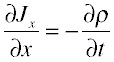
Current and charge are related by the requirement of charge conservation. If current is not constant along a fixed cross-section (like a wire), charge must accumulate. When the current is large coming in (from the left) and small going out (to the right), charge must be accumulating: that is, the time derivative is the opposite in sign of the spatial derivative. In one dimension we can write:
In three dimensions, we need to substitute the divergence for the derivative:
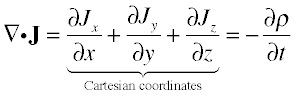
The divergence can also be written in cylindrical or spherical coordinates, as appropriate for the symmetry of a given problem. We will find that this relationship between charges and currents implies a relationship between the resulting potentials, the Lorentz gauge:
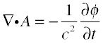
It is computationally rather more elegant to calculate only the vector potential and extract the scalar potential with the Lorentz gauge, but we will generally explicitly exhibit the charge and current distributions and resulting potentials, because it is more intuitive to see where the charges are going, and helps to partition the problem into capacitive and inductive parts.
Celestial Harmonics
It's often very useful to work in the Fourier domain in both space and time, by which we mean that all quantities of interest are assumed to vary in a sinusoidal fashion in time, and to form waves in space. The time and space dependencies are related by the source equations, or equivalently by the requirement that the waves propagate at the speed of light. That is:
where i (or in electrical engineering practice, j) is the imaginary unit (the square root of -1), and the quantity is any of the things we're interested in (a vector or scalar potential). It's easy to see that for plane waves, we must have ω = ck. The virtue of this formalism is, of course, that time derivatives are converted to multiplication by iω, and spatial derivatives become multiplication by -ik when k is a scalar quantity; the vector gradient operator becomes -ik when k is a vector.
Integrals You'll Learn to Love
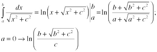
There are a couple of integrals that come up a lot in the source equations, and whose results can be expressed in a tractable analytical form. The first one is going to pop up as soon as we look at a wire. It is:
The second useful integral appears when we look at uniform charges or currents on a planar surface. It is expressed in cylindrical coordinates as:
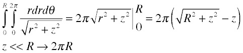
And that's the toolbox for the moment; we're ready to try some real problems.