Dipole Antennas
Daniel M. Dobkin (animation by Nicholas E. Dobkin)
revised May 2013
Bring Your Own Popcorn: Time for a movie...
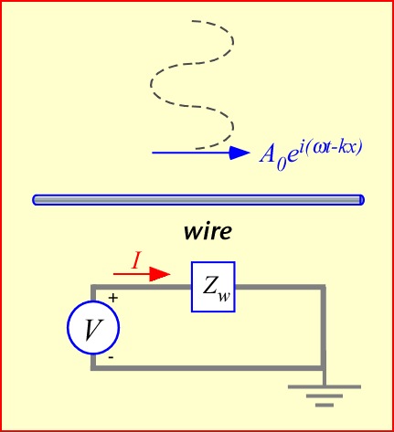
The currents and charges on the surface of a wire antenna adjust themselves to ensure zero electric field inside the antenna. For example, currents flow on a wire to cancel an incident electric field; the resulting induced voltage can be detected by an amplifier and used to receive the signal due to the incident wave. Short antennas behave like capacitors, long antennas like inductors, and at a specific length -- the resonant length, just less than half a wavelength -- the capacitance and inductance cancel, and a large current flows (limited mainly by re-radiation due to the current flow).
To kick things off, we've provided a short Flash animation that illustrates these concepts.
Note that for simplicity we've imagined that positive charges move on the wire, though of course it is normally electrons that do the moving; it's just easier to minimize the number of negative signs that one has to keep track of when trying to explain a concept.
Click here to watch the animation. Hit the BACK button on your browser when you want to return to this page.
Dipole Scaling Arguments
To dig a little deeper, let's return to our wire suspended in space, with an impinging vector potential A and consequent electric field –iωA. For reasonable wire thicknesses, we can assume that currents and charges are only present in a thin layer on the surface of the wire, and adjust themselves to ensure zero field well within the wire. What does this tell us about the distribution of current and charge?
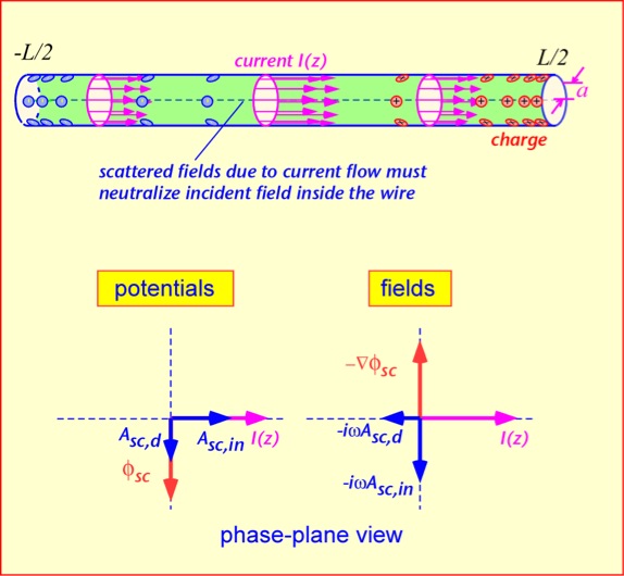
The electric field in the wire arises from the potentials due both to the incident wave and the local charges and currents on the wire. The latter portion is often called the scattered field, though the terminology is perhaps a bit more appealing when our observation point is farther away. To get 0 total field, the scattered field must be equal in magnitude and opposite in direction to the incident field. To see how this comes about it is very helpful to partition the scattered field into three pieces:
- An instantaneous electric potential φsc results from the accumulation of charge, primarily near the ends of the wire, where charge must build up since current cannot flow past the ends. For short antennas we can ignore the time delay between the charge location r’ and the axis of the wire r. The electric field tracks the accumulation of charge in the wire. This is the result of the dipole capacitance.
- An instantaneous magnetic component Asc,in, in phase with the local current, whose value at each location is mainly determined by the current in that vicinity. The electric field lags the current by 90 degrees and so opposes changes in the current: this field is the result of the dipole inductance.
- A delayed magnetic component Asc,d, dependent on the integral of the total current along the wire. For harmonic time dependence, this component lags the instantaneous component by 90 degrees – that is, it is along the negative imaginary axis. Note that the consequent electric field is in phase but directly opposed to the current flow, suspiciously like a conventional resistor. We will find that this is the contribution that leads to the radiation resistance of the antenna.
(There is also a delayed contribution to the scattered electric potential: it is smaller than that due to the magnetic potential because the contributions of the positive and negative charge cancel to first order, so we can neglect it in a qualitative examination; however, it must be included to obtain accurate estimates of the radiation resistance.)
Corresponding to each scattered potential and field we can define an induced voltage. Working in terms of voltages may be more familiar for circuit-type people, and lends itself to approximate calculations rather more gracefully than focusing on fields. We shall somewhat arbitrarily choose to measure this voltage from left to right, in the same direction in which we define the current to be positive. (This is an electrical engineer's view: the voltage across a resistor is measured from the current source to the current sink.) The electrostatic voltage is thus the difference in scalar potential between the left and right sides of the wire, and the magnetic components are the line integrals of the corresponding electric fields along the wire. These three contributions are combined to obtain the net scattered voltage; we then arrange the phase and amplitude of the current so that this scattered voltage approximately cancels the incident voltage Vinc, ensuring that the interior of the wire is field-free as it must be.
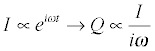
In the movie we asserted that the different contributions scale in different ways as the wire length changes. Let's put some meat on those bones by getting some very rough ideas of how the voltages depend on current and length. The first contribution is the instantaneous scattered potential due to the charges. The charge is just the accumulation of the current; if the current were constant in time we'd have:

In the general case the current is the time derivative of the charge; for a harmonic time dependence we get:
If we treat this charge as a sort of lump at the end of the wire, the rough magnitude of the potential it creates can be gotten from Coulomb's law:
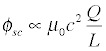
where in the interests of simplicity we're blithely ignoring details like exactly where the charge is and where we're measuring the potential. If this bothers you, have a beer and try again. We plug in the harmonic expression for the charge and find:
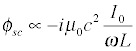
That looks a bit obscure but if we remember that the frequency is related to the wavelength (ω = 2 π c/ λ) we can write this expression in a very appealing fashion:
Here we've defined a sort of characteristic voltage V0 = IZ0, as the product of the current and the characteristic impedance of free space, Z0 =μ0c= 377 ohms. So the antenna voltage due to the charge accumulation scales as the ratio of wavelength to the antenna size, multiplied by this characteristic voltage associated with the current but not with the antenna geometry.
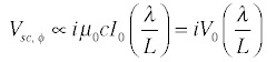
The vector potential due to the current comes from an integral very similar to that we did to estimate inductance, so we’d expect a logarithmic factor in length for A. The voltage is then the derivative (which multiplies the result by the factor iω) multiplied by the length of the wire.
Thus, the voltage due to the current has the opposite sign to that from the charge, and grows instead of shrinking with increased antenna length. We can expect (as posited in the movie) that there will exist a length where the two contributions cancel, and the amount of current flow needed to cancel an incident field is greatly increased: this is the resonant antenna length. To compute the actual current at resonance, it turns out you have to account for the delayed part of the potential (which is ignored above).
Close and Why Did You Want a Cigar, Anyway?
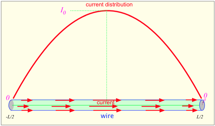
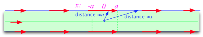
We can get some semi-quantitative results using pretty basic math. We start with just a simple wire of length L and radius a. We’ll use the simplest possible current distribution that has the right properties:
where x=0 in the middle of the wire, as shown in the figure. Recall that the current is flowing on the surface of the wire, and we are requiring that the total fields go to zero at the center of the wire (which is presumed to be thick compared to the skin depth of the current). The current is maximized in the middle of the wire, and goes to 0 at the ends (the charge carriers have nowhere else to go!).
What is the electric field at the middle of the wire (x=0) due to the current and charge?
The charge, as outlined above, is obtained from the derivative of the current:
We then integrate over the sources to find the potentials in the center of the wire (along its axis). Here we make an approximation that greatly simplifies the computation: for x > a or x<-a, we ignore the distance from the axis of the wire to the surface, so the distance r just becomes either x or -x. For |x|<a, we ignore the lateral displacement x, and approximate the distance as about a/1.41. (In the case of the electrostatic potential computation, the charge is 0 near the center anyway, so this part of the integral can simply be neglected.)
We get:
The resulting electric field is:
The electric field at the center due to the charges is similarly found (we skip a step by using the direct source integral for the field):
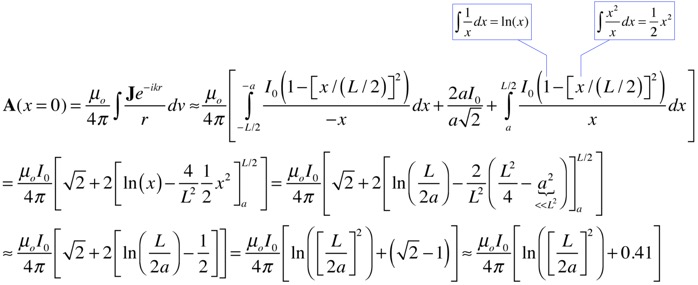
Note that both have essentially the same logarithmic dependence on the wire size for large values of L/a, and opposite dependence on the wavelength. They are of opposite sign, so there will be some ratio of wire length to wavelength at which they are equal, and the total electric field due to both charge and current (but ignoring the phase delay) will be 0:
This is pretty close to the correct answer (about 0.49), accomplished with only the integration of (1/x) and x.
At resonance, the field does not go to 0, or the current needed to cancel an incident field would be infinite! But to find it, we have to incorporate the phase delay between the sources at the ends of the wire and the field at the center, at least to first order. We expand the complex exponential:
and find the magnetic vector potential due to the first-order term, again setting r=x for x>a:
This is the field resulting from the current I0 when the length of the antenna is such that the imaginary contributions vanish: that is, the antenna is resonant. For a given incident field, we can find the current:
If we turn the wire into a dipole antenna, by slicing it in half in the middle and making contact to each wire, this is the current we will measure when we present a short circuit to the antenna. If we know the short-circuit current (which we just derived above) and the open-circuit voltage, we can obtain the equivalent circuit of the antenna.
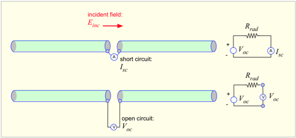
A very simple approach to obtaining the open-circuit voltage is to realize that the field on the antenna must be equal to the incident field in magnitude, and opposite in sign. Since the field extends across each half of the dipole, the resulting voltage is:
(This is a bit of an oversimplification, since the voltage on the antenna arises only from the electrostatic part of the field, whereas it is the total field, with magnetic contribution, that matches the incident field.)
By taking the ratio of the voltage and current we obtain the equivalent resistance -- the radiation resistance -- of the antenna:
For our estimate of the resonant length of the antenna relative to a wavelength, this is about 80 ohms -- around 20% higher than the actual answer for a real antenna with reasonably high (L/a).
So we’ve obtained fairly accurate answers for the impedance of the antenna without having to do anything more complicated than the integral of (1/x). And once again, we have found no need to compute the magnetic field B in doing so.
For a more detailed derivation of the impedance of a short antenna, you can read the article linked here.