A More Elaborate (but still approximate) Derivation of the Self-Inductance of a Loop
Dan Dobkin
revised December 2012
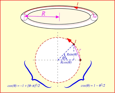
To find the self-inductance of a circular loop, we need to find the vector potential pointing in the direction of the wire (that is, tangential to the circular loop). By symmetry we only need to find the potential at one point around the loop, but we need to integrate over the currents flowing around the whole loop. We can express position around the loop in terms of the central angle, θ; the coordinates of a point on the loop are proportional to the cosine and sine of the angle. We need to remember to multiply the angular differential by the radius to create a line integral around the loop. Here's the loop:

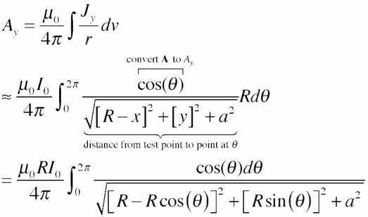
Without loss of generality we can let the test point (where we're finding the potential) be located at y=0. We will formulate the integral by finding the expression for distance from the test point to a point on the loop, and then approximate the cosine in two parts: when we are on the same side of the circle, cosine falls quadratically away from 0, and when on the other side cosine grows quadratically towards the opposite end. (We'll see in a moment that no such approximation is needed for the sine.) As long as the radius of the wire is much less than the loop radius, we can ignore the fact that the distance to the inner surface of the wire (facing the center of the loop) is slightly less than that to the outer surface. We will again assume constant current around the loop and integrate over the current to find the potential. The first step is to write everything out:

Here the cosine on the top arises because the vector A always points in the direction of the loop (where the current is going), but we're trying to find the component of A in the y-direction -- that is, along the wire at the test point, y= 0. The last expression is obtained by substituting for the sine and cosine. This integral looks pretty ugly but let's charge ahead by multiplying out the squares in the denominator:

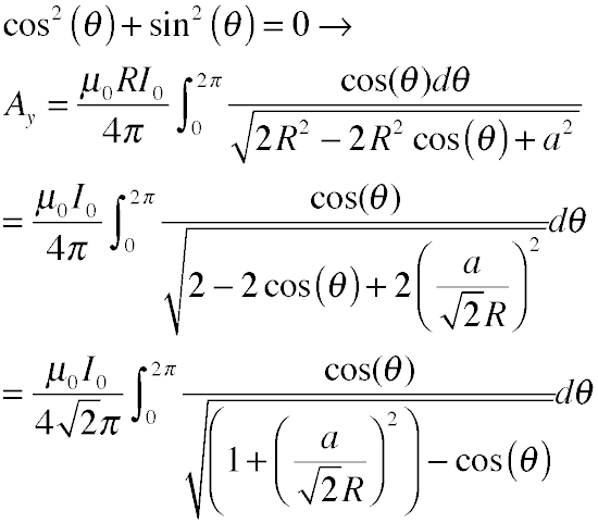
Now use the fact that the square of cosine and sine make 1:

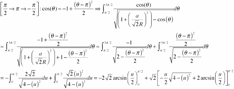
This is the surprisingly nasty integral that leads to hypergeometric gobblydegook. So here's where we apply our approximation for the cosine. First split the integral into nearby and distant halves:

Now approximate the cosine: first on the nearby half...

resulting in:

and for the distant half:

finally obtaining:

We add these two contributions together and fold the constants into the logarithm to get the tangential vector potential:

By symmetry, the potential is the same all around the loop, so the inductance around the loop is obtained by just multiplying by the perimeter, and dividing by the current. We get:

which was rather a lot of work to get a tiny change in a numerical factor inside a logarithm! We can extract some extra benefit from our pain by formulating a few rules of thumb:
- near the test point on a wire, the potential just looks like that of a straight wire
- regions of the wire that point away from the current tangential direction don't do much
- distant regions of the wire don't have to be treated accurately: the distance can be approximated as constant, and the radius of the wire can be neglected.
Just for completeness, let's see how our answers perform. Below we compare the performance of the full integration, the single-point integration for the equivalent square coil, the "standard" approximate formula for loop inductance, and a numerical integration of the source integral:
R | a | R/a | this work | standard | 1-point | numerical | error (this) | error (1pt) | error (std) |
1 | .05 | 20 | 3.8 | 3.8 | 3.7 | 3.9 | -1% | -6% | -3% |
| 1 | 0.02 | 50 | 5 | 4.9 | 4.9 | 5 | -1% | -2% | -2% |
| 1 | 0.005 | 200 | 6.7 | 6.7 | 6.6 | 6.8 | -1% | -3% | -2% |
(The standard formula comes from Finkenzeller's RFID Handbook, equation 4.12. The numerical calculation is numerical integration of the potential due to a single circular loop of current displaced by a above a test point, so it is accurate for large values of R/a, and addresses the quality of the cosine approximation. )
If you want an accurate answer you need to integrate the source equation, but if you're trying to get within 5%, the “equivalent square” model works pretty well and is a lot simpler to implement and to understand.
